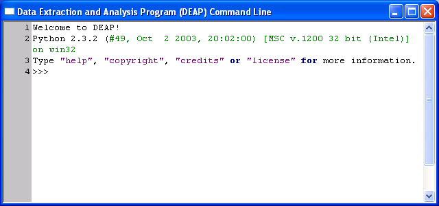
All functionality of DEAP is available via the command line interface. A picture of a typical command line window is illustrated below:
All of the syntax at the command line follows Python conventions. All of the parameters passed to each one of the operations can either be passed using the name of the parameter and in any order (e.g. text = "my text"), or in the exact order specified below but without the parameter name. Also, all of the native Python syntax is available at the command line. More information about Python and its syntax is available here.
AddDeviceAnnotation(side = string, disp = number, coord = number, fjust = number, text = string)
This command adds an annotation to the currently active panel. The annotation will resize when the axes are rescaled. The command returns an integers which is a unique annotation index.
side may be on of the following strings: 'B', 'L', 'LV', 'T', 'R' or 'RV'; these strings mean bottom, left, left vertical, top, right, and right vertical respectively. side determines which panel edge is referenced when locating the annotation. disp indicates a displacement from the specified panel edge. coord indicates the location of the annotation on the specified panel edge. fjust controls annotation justification. When fjust is 0.0, the annotation is left-justified. When fjust is 0.5, the annotation is centered. When fjust is 1.0, the annotation is right-justified. Other values for fjust between 0.0 and 1.0, use an intermediate placing. text is the annotation string.
This command adds an annotation to the currently active panel. The annotation will not resize nor move as the axes are rescaled. The command returns an integer which is a unique annotation index.
The color of the text and the text background must be an integer between 0 and 15 inclusive. The following map details the color assigned to each integer value.
0 = black, 1 = white, 2 = red, 3 = green, 4 = blue, 5 = cyan, 6 = magenta, 7 = yellow, 8 = orange, 9 = green-yellow, 10 = green-cyan, 11 = blue-cyan, 12 = blue-magenta, 13 = red-magenta, 14 = dark gray, 15 = light gray
This command makes the newly added panel the currently active panel and returns an integer which is a unique panel index. Each panel has its own set of axes, title, and plots. The first image below shows one empty panel and the second shows two empty panels.


AddXYErrorBars(lower = list, upper = list, color = int)
This command adds error bars to the currently active plot. The first list is a set of the lower limits, with a one-to-one relationship with the data points on the graph. The second list specifies the upper limits. The third parameter is an integer to specify the color of the error bars.
The color of the error bars must be an integer between 0 and 15 inclusive. The following map details the color assigned to each integer value.
0 = black, 1 = white, 2 = red, 3 = green, 4 = blue, 5 = cyan, 6 = magenta, 7 = yellow, 8 = orange, 9 = green-yellow, 10 = green-cyan, 11 = blue-cyan, 12 = blue-magenta, 13 = red-magenta, 14 = dark gray, 15 = light gray
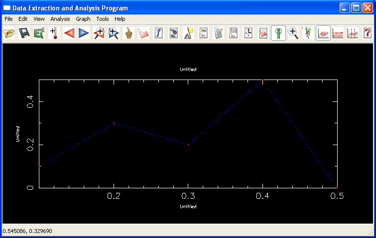
The most fundamental command is to add an XY Plot to the graph. As the name implies, an XY plot is just a group of X and Y data, plotted on the XY axes. The syntax is to supply two lists, one of X data and one of Y data, each list within square brackets. Both lists must be of the same length. An example is as follows:
i = AddXYPlot([.1, .2, .3, .4, .5], [.1, .3, .2, .5, 0])
There can be more than one XY plot on the graph at any one time. The number that gets returned by the function is assigned to i, and is the index of the newly added plot. The newly added plot becomes the active plot automatically. For large X and Y lists, the user should assign those lists to variables and then pass the variables into the function. An example is as follows:
x = [.1, .2, .3, .4, .5]
y = [.1, .3, .2, .5, 0]
i = AddXYPlot(x, y)
An example of the plot added to the display is illustrated below:
This command divides the currently active plot into an equal number of bins specified by the argument. The extents of the bin are defined by the minimum and maximum X values in the data set or data sets on the plot. The data points are then assigned to the bins and can be retrieved via GetXYBinX() and GetXYBinY(). For example if a data set ranged from (1, 2) to (5, 1) and one wishes to create two bins, the first bin will be defined as [1, 3) and the second bin will be [3, 5]. Data points with X values where 1 <= x < 3 will be placed in bin 1 and data points with X values where 3 <= x <= 5 will be placed in bin2.
Removes all plots and plot information. This action cannot be undone.
This command exports the data currently in the graphical display to the file specified in the parameter to JPG, PNG, Bitmap, Postscript, or color Postscript formats. The format is specified via the filename parameter. The filename string must end in either .jpg, .png, .bmp, .ps, or .cps.
Flag(value = int, flagColor = int, flagShow = int)
This command changes the properties associated with data point having the given flag value. flagColor is an integer specifying the color of the data points with the given flag value. flagShow is an integer where 0 indicates to hide the data points associated with a given flag value and 1 indicates to display the data points associated with a given flag value.
The color of the flagged data must be an integer between 0 and 15 inclusive. The following map details the color assigned to each integer value.
0 = black, 1 = white, 2 = red, 3 = green, 4 = blue, 5 = cyan, 6 = magenta, 7 = yellow, 8 = orange, 9 = green-yellow, 10 = green-cyan, 11 = blue-cyan, 12 = blue-magenta, 13 = red-magenta, 14 = dark gray, 15 = light gray
This command is meant to be called in user-created scripts. It can be called at any point in the script to suspend further processing of script commands and allow the user to view/interact with the plot that has been created up to that point. The execution of the script can be resumed by calling Unfreeze from DEAP's plot window. The message string can be used to print text in the Freeze dialog box.
This command performs a Gaussian fit on the currently active plot and returns the peak, center, and height of the fitted Gaussian. A Gaussian fit attempts to find the Gaussian function which best describes the data set being fitted.
This function returns the plot index of the currently active plot.
This function returns the text of the indexed annotation.
This command returns the caption of the currently active plot.
This function returns a list of (integer) flags associated with each data point in the active data set.
This function returns the number of annotations contained on all the panels.
This function returns the number of plots that are on the currently active panel.
Returns the number of bins last created by BinXYData for the currently active plot.
This command returns whether or not the legend is currently being displayed on the currently active panel in the DEAP plot window. A return value of 1 indicates that the legend is currently being displayed on the panel and a value of 0 indicates that the legend is not currently being displayed on the panel.
This command returns a Text object which contains the title information for the currently active panel. A Text object has the following attributes: text, font, color, size, and bgColor. The following is an example of how to use this command:
title = GetTitle()
print title.text, title.font, title.color, title.size, title.bgColor
This function returns the X data list for the active plot.
Returns the binned X values for the currently active plot. The return value is a list of lists. Each sublist contains the X values for a particular bin.
Returns the binned Y values for the currently active plot. The return value is a list of lists. Each sublist contains the Y values for a particular bin.
This function returns the Y data list for the active plot.
This command performs a linear fit on the currently active plot and returns the y-intercept and slope of the fitted line. A linear fit attempts to find the line which best describes the plot data being fitted.
This function returns the mean value of the data in the currently active plot.
ModifyXYPlot(index = int, x = list, y = list)
This command modifies the data set contained in the specified active plot. The first argument is the index of the plot that is to be modified. The list of X and Y data is formatted as in AddXYPlot -- A list of numbers, separated by commas, within square brackets. If a set of X or Y data does not need to be modified, use the keyword "None".
The following example changes the X data for plot 0, but leaves the Y data unchanged:
ModifyXYPlot(0, [.1, .3, .2, .5, 0], None)
This command performs a polynomial fit on the currently active plot and returns the coefficients of the fitted polynomial. n is the degree of the polynomial to be fitted to the active plot. A polynomial fit attempts to find a polynomial function of the specified degree which best describes the data set being fitted.
This function repeats the previous command.
This command removes the specified annotation from the display.
This command removes the specified plot from the plotting window.
This command undoes the effects of the SuspendUpdates command, which directs the application to redraw the plots after each plot update.
This command activates the indicated plot. All future plot specific commands will be made to this plot by default.
SetCaption(text = string, index = int)
This command associates a caption with a specified plot. The first argument is the text of the caption and the second is the index of the plot with which the caption is associated.
This command sets the flag values for each point in the active data set. The length of flags must be of the same length as the active data set, i.e. there is one flag value per data point.
SetTitle(title = string, font = int, color = int, size = int, bgcolor = int)
This command sets the title for the active panel on the plot window. The font, color, and bgColor of the title are specified by integer numbers. These values are mapped below:
Font:
1 = normal, 2 = roman, 3 = italic, 4 = script
Color, bgColor:
0 = black, 1 = white, 2 = red, 3 = green, 4 = blue, 5 = cyan, 6 = magenta,
7 = yellow, 8 = orange, 9 = green-yellow, 10 = green-cyan, 11 = blue-cyan,
12 = blue-magenta, 13 = red-magenta, 14 = dark gray, 15 = light gray
An example of how to use the SetTitle command is as follows:
SetTitle("Example Plot", font = 4, size = 2, color = 2)
This command modifies the X axis displayed on the plotting window. xMin and xMax specify the minimum and maximum values of the axis respectively. type may be either "linear", "log", or "time". autoscale can either be 0 or 1; 0 indicates that the Y1 axis should automatically scale itself to fit the data displayed on the panel (ignoring yMin and yMax) and a 1 indicates that the Y1 axis should use yMin and yMax as its extents. text specifies the axis label and font, color, size, and bgColor format the axis label. The possible values of font, color, and bgColor are shown below:
Font:
1 = normal, 2 = roman, 3 = italic, 4 = script
Color, bgColor:
0 = black, 1 = white, 2 = red, 3 = green, 4 = blue, 5 = cyan, 6 = magenta,
7 = yellow, 8 = orange, 9 = green-yellow, 10 = green-cyan, 11 = blue-cyan,
12 = blue-magenta, 13 = red-magenta, 14 = dark gray, 15 = light gray
SetXYErrorBarColor(color = int)
This command changes the color of the error bars on the currently active plot.
The following color map shows the possible integer values of color:
0 = black, 1 = white, 2 = red, 3 = green, 4 = blue, 5 = cyan, 6 = magenta, 7 = yellow, 8 = orange, 9 = green-yellow, 10 = green-cyan, 11 = blue-cyan, 12 = blue-magenta, 13 = red-magenta, 14 = dark gray, 15 = light gray
SetXYLinePattern(pattern = int, width = int, color = int)
This command modifies the type of line connecting the data points on the plot. The user can choose to have no line displayed at all by setting the pattern to 0 (zero). The following line patterns are available: 0 = no line, 1 = solid line, 2 = dashed line, 3 = dot-dash, 4 = dotted, 5 = dash-dot-dot-dot. width controls the width of the displayed line. Valid values for line color are 0 through 15 as shown in the map below:
0 = black, 1 = white, 2 = red, 3 = green, 4 = blue, 5 = cyan, 6 = magenta, 7 = yellow, 8 = orange, 9 = green-yellow, 10 = green-cyan, 11 = blue-cyan, 12 = blue-magenta, 13 = red-magenta, 14 = dark gray, 15 = light gray
SetXYMarker(marker = int, colors = int)
This command modifies the color and representation of each data point in a data set on the plot. Valid marker values are -6 through 31 inclusive. Valid values for color are 0 through 15 inclusive as shown below:
0 = black, 1 = white, 2 = red, 3 = green, 4 = blue, 5 = cyan, 6 = magenta, 7 = yellow, 8 = orange, 9 = green-yellow, 10 = green-cyan, 11 = blue-cyan, 12 = blue-magenta, 13 = red-magenta, 14 = dark gray, 15 = light gray
To indicate the no markers are to be drawn, enter None for the marker type. The following chart displays the marker symbols associated with the integer marker values:
This command modifies the Y1 axis displayed on the plotting window. yMin and yMax specify the minimum and maximum values of the axis respectively. type may be either "linear", "log", or "time". autoscale can either be 0 or 1; 0 indicates that the Y1 axis should automatically scale itself to fit the data displayed on the panel (ignoring yMin and yMax) and a 1 indicates that the Y1 axis should use yMin and yMax as its extents. text specifies the axis label and font, color, size, and bgColor format the axis label. The possible values of font, color, and bgColor are shown below:
Font:
1 = normal, 2 = roman, 3 = italic, 4 = script
Color, bgColor:
0 = black, 1 = white, 2 = red, 3 = green, 4 = blue, 5 = cyan, 6 = magenta,
7 = yellow, 8 = orange, 9 = green-yellow, 10 = green-cyan, 11 = blue-cyan,
12 = blue-magenta, 13 = red-magenta, 14 = dark gray, 15 = light gray
This command toggles the legend display on the currently active panel. A value of 1 indicates to display the legend and a value of 0 indicates to hide the legend.
This command toggles the display of the error bars for the currently active plot. A value of 1 indicates to display the error bars and a value of 0 indicates that the error bars should be hidden.
This command returns the standard deviation of the data contained in the currently active plot.
This command undoes the effects of the previous command.
There are several syntatatic nuances to the command line interface that are tough to explain. The command line is meant to mimic the typical use of the Python command line interpreter, but with functions specifically implemented for DEAP. If the user has experience with Python, then the command line will be easy to pick up. If not, there will be a little more learning involved. The following is a transcript of how a typical session with DEAP may look, what the syntax of the commands is, and what the outputs of the commands would be.
>>> i = AddXYPlot([.1, .2, .3, .4, .5], [.1, .3, .2, .5, 0])
>>> print "Newly added plot index is: ", i
Newly added plot index is: 0
>>> print "The number of plots is: ", GetNumPlots()
The number of plots is: 1
>>> print "The active plot is: ", GetActivePlot()
The active plot is: 0
>>> SetTitle("Example Plot", font = 4, size = 2, color = 2)
>>> print "The new title is: ", GetTitle().text
The new title is: Example Plot
>>> j = AddXYPlot([.5, .3, .2, .1, .4], [.2, 0, .1, .4, 0.3])
>>> print "The active plot is: ", GetActivePlot()
The active plot is: 1
>>> RemovePlot(j)
>>> print "The active plot is: ", GetActivePlot()
The active plot is: 0
>>> ModifyXYPlot(i, [.1, .3, .4, .5, .6], [.2, 0, .1, .4, 0.3])
>>> print "x = ", GetXData()
x =  [0.10000000000000001, 0.29999999999999999, 0.40000000000000002, 0.5, 0.59999999999999998]
>>> print "y = ", GetYData()
y =  [0.20000000000000001, 0, 0.10000000000000001, 0.40000000000000002, 0.29999999999999999]
>>> SetXYMarker(15, 3)
>>> SetXYLinePattern(1, 1, 7)
>>> AddXYErrorBars([.05, .02, .01, .03, .04],[.03, .01, .02, .04, .05])
>>> SetXYErrorBarColor(9)
>>> ShowXYErrorBars(0)
>>> ShowXYErrorBars(1)
>>> BinXYData(2)
>>> print "Bin X = ", GetXYBinX()
Bin X =  [[0.10000000000000001, 0.29999999999999999], [0.40000000000000002, 0.5, 0.59999999999999998]]
>>> print "Bin Y = ", GetXYBinY()
Bin Y =  [[0.20000000000000001, 0], [0.10000000000000001, 0.40000000000000002, 0.29999999999999999]]
>>> print GetNumXYBins()
2
>>> Export("test.bmp")
>>> k = AddWorldAnnotation(text = "nifty new annotation", xPos = 0.2, yPos = 0.2)
>>> RemoveAnnotation(k)
>>> AddWorldAnnotation(text = "more annotation", xPos = 0.4, yPos = 0.4)
>>> SetCaption("better data set name")
>>> print GetCaption()
better data set name
>>> ShowLegend(1)
>>> print "GetShowLegend() = ", GetShowLegend()
GetShowLegend = 1
The other mode of DEAP operation is to invoke commands using the plot window This mode is used for plot interaction activities, e.g. data flagging. Almost all of the operations from the plot window map exactly to the command line functionality.
 Annotate. This command allows the user to create and place an annotation
through the use of the annotation dialog box displayed below.
Annotate. This command allows the user to create and place an annotation
through the use of the annotation dialog box displayed below.
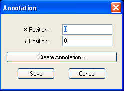
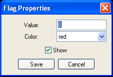
The user can set the text, height, font, color, and background color for the annotation. The command GetNumAnnotations can be used at the command line to retrieve the number of existing annotations, and RemoveAnnotation can be used to remove annotations from the plot.
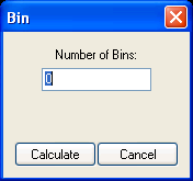
 Bin. This command allows the user to divide the active data set into an equal
number of bins specified in the bin dialog window. For additional information,
refer to the BinXYData command.
Bin. This command allows the user to divide the active data set into an equal
number of bins specified in the bin dialog window. For additional information,
refer to the BinXYData command.
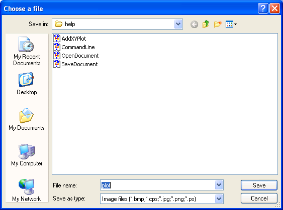
 Export. Selecting this button calls up the export file dialog and allows the
user to save only the graphics to a file. Supported graphical formats are:
bitmap, color Postscript, JPG, PNG, and Postscript.
Export. Selecting this button calls up the export file dialog and allows the
user to save only the graphics to a file. Supported graphical formats are:
bitmap, color Postscript, JPG, PNG, and Postscript.
 Fit. This dialog allows the user to fit the currently active data set to
a mathematical function. Functions that are currently available are:
linear fit, polynomial fit (to a specified degree), and Gaussian fit.
Fit. This dialog allows the user to fit the currently active data set to
a mathematical function. Functions that are currently available are:
linear fit, polynomial fit (to a specified degree), and Gaussian fit.
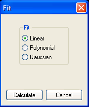
A linear fit on the currently active plot returns the y-intercept along with the slope of the fitted line.
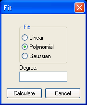
A polynomial fit to a specified degree on the currently active plot returns the coefficients of the fitted polynomial. Selecting the polynomial fit option reveals an input field for the degree associated with the polynomial as show in the image below.
A Gaussian fit on the currently active plot and returns the peak, center, and height of the fitted Gaussian.
 Flag Properties. This command allows the user to change the properties
associated with data points having the given flag value.
Flag Properties. This command allows the user to change the properties
associated with data points having the given flag value.
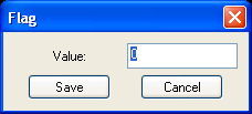
 Flag Tool. The Flag Tool allows the user to enter the flag value to be
associated with the subsequent lasso operations. Once a value has been entered
and saved, use the mouse pointer to enclose all data points that are to be
flagged with the entered value.
Flag Tool. The Flag Tool allows the user to enter the flag value to be
associated with the subsequent lasso operations. Once a value has been entered
and saved, use the mouse pointer to enclose all data points that are to be
flagged with the entered value.
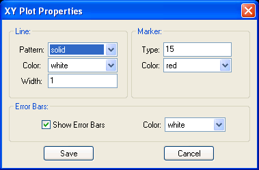
 Graph Properties. This command brings up the plot properties dialog box, which
consists of three sections: Line, Marker, and Error Bars.
In the Line section, the pattern, color, and width of the line connecting each
data point in the plot can be specified. The options in the Marker section
determine the type and color of the markers indicating each data point.
Under the Error Bars section,
the user can select to show or hide the error bars, and assign a color to
them. Error bar data must be entered via the command line by using the
AddXYErrorBars command.
Graph Properties. This command brings up the plot properties dialog box, which
consists of three sections: Line, Marker, and Error Bars.
In the Line section, the pattern, color, and width of the line connecting each
data point in the plot can be specified. The options in the Marker section
determine the type and color of the markers indicating each data point.
Under the Error Bars section,
the user can select to show or hide the error bars, and assign a color to
them. Error bar data must be entered via the command line by using the
AddXYErrorBars command.
The colors must be an integer between 0 and 15 inclusive. The following map details the color assigned to each integer value.
0 = black, 1 = white, 2 = red, 3 = green, 4 = blue, 5 = cyan, 6 = magenta, 7 = yellow, 8 = orange, 9 = green-yellow, 10 = green-cyan, 11 = blue-cyan, 12 = blue-magenta, 13 = red-magenta, 14 = dark gray, 15 = light gray
To indicate the no markers are to be drawn, enter None for the marker type. The following chart displays the marker symbols associated with the integer marker values:
 Info Tool. This tool allows the user to see the world coordinates corresponding
to the cursor position on the plot in the status bar at the bottom of the plot
window.
Info Tool. This tool allows the user to see the world coordinates corresponding
to the cursor position on the plot in the status bar at the bottom of the plot
window.
 Legend. This command invokes the legend dialog box. The user can modify
the captions for each data set and indicate whether or not the legend is to
be displayed on the plot window.
Legend. This command invokes the legend dialog box. The user can modify
the captions for each data set and indicate whether or not the legend is to
be displayed on the plot window.

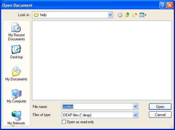
 Open. Selecting this button calls up the open file dialog and allows the
user to retrieve previously saved DEAP sessions (.deap files).
Open. Selecting this button calls up the open file dialog and allows the
user to retrieve previously saved DEAP sessions (.deap files).
 Redo. This command redoes your last command. When there are no commands in
the redo history that can be redone, the Redo command in the menu bar will be
grayed and clicking the Redo icon will result in no action.
Redo. This command redoes your last command. When there are no commands in
the redo history that can be redone, the Redo command in the menu bar will be
grayed and clicking the Redo icon will result in no action.
 Rezoom. The Rezoom command redoes a previously executed zoom command.
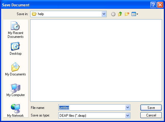
 Save. Selecting this button calls up the save file dialog and allows the
user to save the current session to a .deap file. All graphics and data
are saved.
Save. Selecting this button calls up the save file dialog and allows the
user to save the current session to a .deap file. All graphics and data
are saved.
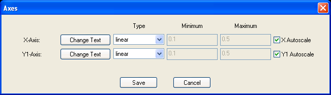
 Scale Axes. This dialog provides the user with the ability to change the axes
of the plot. The user can change the text, type, and scaling for each axis.
The Change Text button results in the same text change dialog as for
annotations and title, providing the ability to change the text, font, height,
color, and background color. The type of the axes can be linear,
logarithmic or time. The user may also choose to have the axes autoscaled, or
specify minimum and maximum values for each axis.
Scale Axes. This dialog provides the user with the ability to change the axes
of the plot. The user can change the text, type, and scaling for each axis.
The Change Text button results in the same text change dialog as for
annotations and title, providing the ability to change the text, font, height,
color, and background color. The type of the axes can be linear,
logarithmic or time. The user may also choose to have the axes autoscaled, or
specify minimum and maximum values for each axis.
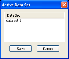
 Select Active Data Set. A DEAP plot can contain multiple data sets.
The active data set dialog allows for selection of the current active data set.
While all data sets may be displayed, only the selected active data set will
be affected by, or taken into consideration, for plot-specific commands.
Select Active Data Set. A DEAP plot can contain multiple data sets.
The active data set dialog allows for selection of the current active data set.
While all data sets may be displayed, only the selected active data set will
be affected by, or taken into consideration, for plot-specific commands.
 Select Box. This tool allows the user to select a region of the plot
enclosed by a box. In this mode, all lasso operations will be performed in
form of a rectangular box.
Select Box. This tool allows the user to select a region of the plot
enclosed by a box. In this mode, all lasso operations will be performed in
form of a rectangular box.
 Select Horizontal Bars. Allows the user to select a region of the plot
enclosed by horizontal lines. In this mode, all lasso operations will be
performed in form of a pair of horizontal bars.
Select Horizontal Bars. Allows the user to select a region of the plot
enclosed by horizontal lines. In this mode, all lasso operations will be
performed in form of a pair of horizontal bars.
 Select Vertical Bars. Allows the user to select a region of the plot enclosed
by vertical lines. In this mode, all lasso operations will be performed in
form of a pair of vertical bars.
Select Vertical Bars. Allows the user to select a region of the plot enclosed
by vertical lines. In this mode, all lasso operations will be performed in
form of a pair of vertical bars.
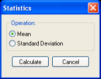
 Statistics. This dialog allows the user to apply a statistical calculation
to the currently active plot. The two calculations that are available are
mean and standard deviation.
Statistics. This dialog allows the user to apply a statistical calculation
to the currently active plot. The two calculations that are available are
mean and standard deviation.
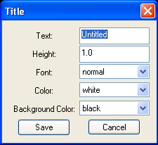
 Title. This command allows the user to change the title of the plot.
The user change the text, height, font, color, and background color of the
title.
Title. This command allows the user to change the title of the plot.
The user change the text, height, font, color, and background color of the
title.
 Undo. This command undoes your last command. Please note that DEAP includes
operations that cannot be undone. When there are no commands in the undo
history that can be undone, the Undo command in the menu bar will be grayed
and clicking the Undo icon will result in no action.
Undo. This command undoes your last command. Please note that DEAP includes
operations that cannot be undone. When there are no commands in the undo
history that can be undone, the Undo command in the menu bar will be grayed
and clicking the Undo icon will result in no action.
 Unfreeze. This command unfreezes the processing of commands via the command
line. This command is intended for use in conjunction with the
Freeze command. The Freeze command is called at any
point in a script to suspend further processing of script commands and allow
the user to view/interact with the plot that has been created to that point.
The Unfreeze command is invoked to resume operation.
Unfreeze. This command unfreezes the processing of commands via the command
line. This command is intended for use in conjunction with the
Freeze command. The Freeze command is called at any
point in a script to suspend further processing of script commands and allow
the user to view/interact with the plot that has been created to that point.
The Unfreeze command is invoked to resume operation.
 Unzoom. The Unzoom command undoes a previously executed zoom command.
 User Manual. The User Manual button displays the DEAP User Manual.
 Zoom Tool. Selecting the zoom tool allows the user to use the mouse pointer
for zooming in on a particular area of the plot.
Zoom Tool. Selecting the zoom tool allows the user to use the mouse pointer
for zooming in on a particular area of the plot.
As displayed in the screen shot below, the menu bar found at the top of the page contains the same commands as found within the toolbar menu with the addition of a few others.

While the icons provide quick, single-click access to GUI functions, the menu bar includes a categorized listing of the functions under menu options File, Edit, View, Analysis, Graph, Tools, and Help.